
2021-12-06

Practice Final Thread .
Please post your solutions to the practice final to this thread.
Best,
Chris
Please post your solutions to the practice final to this thread.
Best,
Chris
Pradeep Narayana, Aditya Singhania
Question 6:
a. Excess error is the amount by which the current cost function is larger than the minimal possible cost. It is given by :
J(θ)-min j(θ)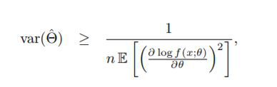
b. If we have two unbiased estimators W1, W2 of the same quantity, we say W1 is more efficient than W2 if Var(W1)<Var(W2). For an unbiased estimator, efficiency indicates how much its precision is lower than the theoretical limit of precision provided by the Cramer-Rao inequality
c. Nesterov Momentum is just like more traditional momentum except the update is performed using the partial derivative of the projected update rather than the derivative current variable value. Here, the gradient is evaluated after the current velocity is applied.
Question 10:
Steps in Ng's NN design methodology:
1) Define goals (e.g., error metrics, target values), depending on the problem statement.
2) Get end-to-end pipeline up and running as soon as possible.
3) Determine main bottlenecks in reaching goals that may be causing over/under-fitting or not converging.
4) Repeatedly make incremental changes (e.g., include additional data, adjust hyperparameters, change algorithms).
Determine your goals - Determine what error metrics to use, and the target values for these metrics.
A few existing common metrics are accuracy, confusion matrix components and ROC curves.
Sometimes we may need more advanced metrics.
Example, in a case where we are classifying mail as spam or genuine, we can use the weighting of the FPR with FNR.
In a case where we want to detect rare events such as detection of cancer, we can use precision(fraction of reportings that are correct) and recall(fraction of true events detected).
These two can be combined as one such as PR curve and F1 score : 2RP/(R+P)
In the street view of Google maps, they used "coverage" which estimated the (total addresses added to map) / (total addresses detected) and played this value versus accuracy.
In an ad placement, AI might use click-through as a metric
(Edited: 2021-12-06) Pradeep Narayana, Aditya Singhania
<u>'''Question 6:'''</u>
a. Excess error is the amount by which the current cost function is larger than the minimal possible cost. It is given by :
J(θ)-min j(θ)
b. If we have two unbiased estimators W1, W2 of the same quantity, we say W1 is more efficient than W2 if Var(W1)<Var(W2). For an unbiased estimator, efficiency indicates how much its precision is lower than the theoretical limit of precision provided by the Cramer-Rao inequality
((resource:cramer.JPG|Resource Description for cramer.JPG))
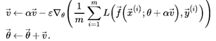
c. Nesterov Momentum is just like more traditional momentum except the update is performed using the partial derivative of the projected update rather than the derivative current variable value. Here, the gradient is evaluated after the current velocity is applied.
((resource:Nesterov.png|Resource Description for Nesterov.png))
<u>'''Question 10:'''</u>
Steps in Ng's NN design methodology:
1) Define goals (e.g., error metrics, target values), depending on the problem statement.
2) Get end-to-end pipeline up and running as soon as possible.
3) Determine main bottlenecks in reaching goals that may be causing over/under-fitting or not converging.
4) Repeatedly make incremental changes (e.g., include additional data, adjust hyperparameters, change algorithms).
Determine your goals - Determine what error metrics to use, and the target values for these metrics.
A few existing common metrics are accuracy, confusion matrix components and ROC curves.
Sometimes we may need more advanced metrics.
Example, in a case where we are classifying mail as spam or genuine, we can use the weighting of the FPR with FNR.
In a case where we want to detect rare events such as detection of cancer, we can use precision(fraction of reportings that are correct) and recall(fraction of true events detected).
These two can be combined as one such as PR curve and F1 score : 2RP/(R+P)
In the street view of Google maps, they used "coverage" which estimated the (total addresses added to map) / (total addresses detected) and played this value versus accuracy.
In an ad placement, AI might use click-through as a metric
Name- Parth Sandip Mehta and Abhishek Vaid
Q8 Answer8-
The Above outlines how to create a custom layer in Keras as done in homework 4.
The above uses the custom layer just created using Keras's functional API.
The source code is taken from homework 4.
Q3) Answer 3)
(Edited: 2021-12-06)
Name- Parth Sandip Mehta and Abhishek Vaid
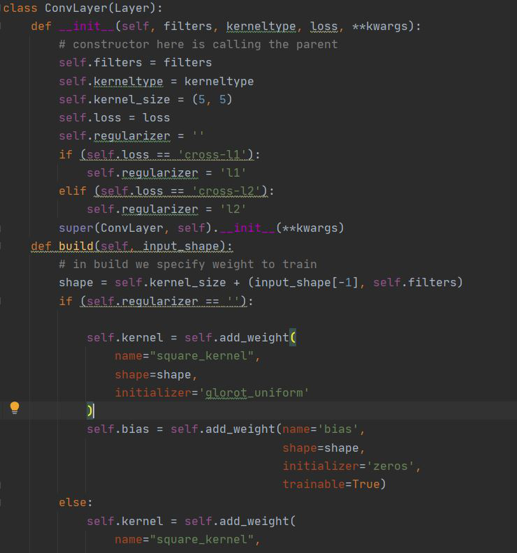
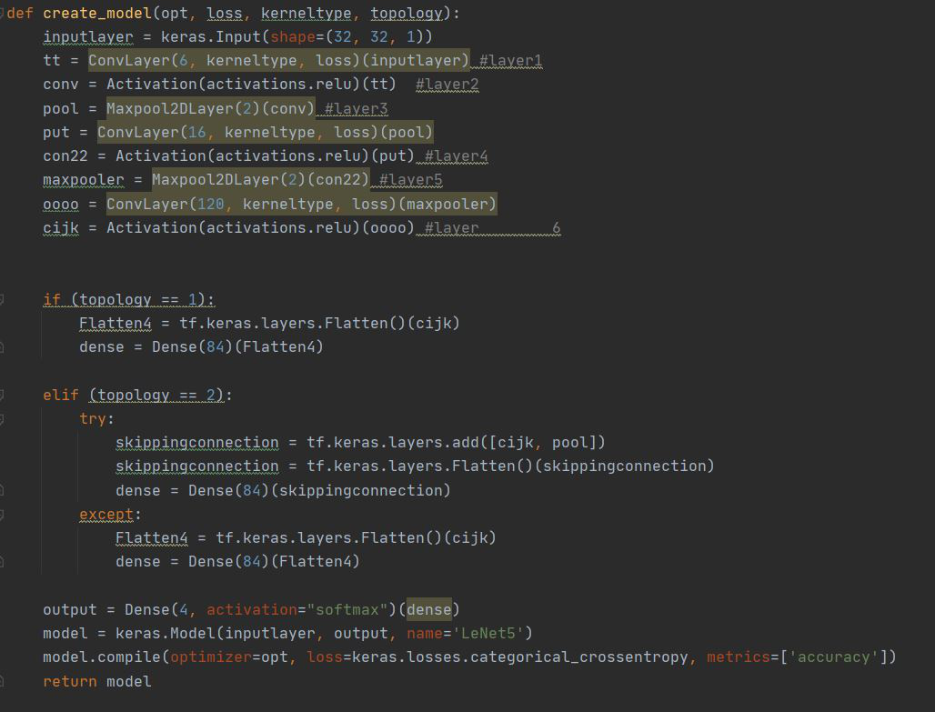
'''Q8 Answer8-'''
((resource:11.JPG|Resource Description for 11.JPG))
((resource:12.JPG|Resource Description for 12.JPG))
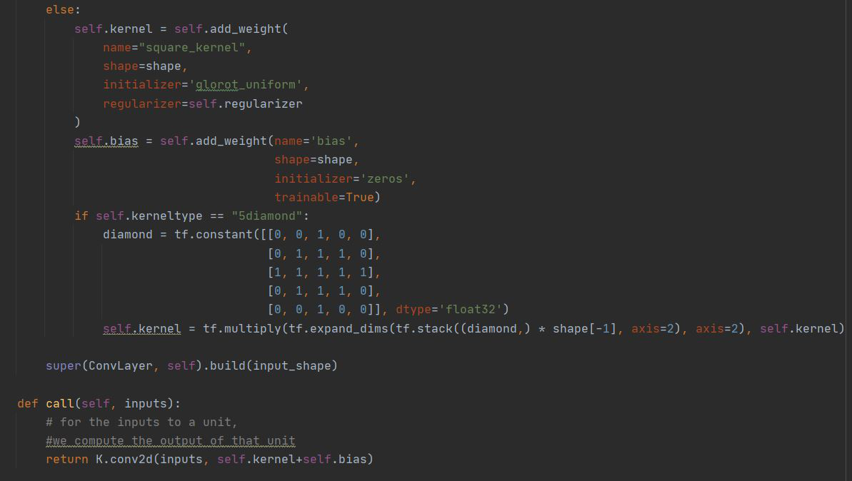
The Above outlines how to create a custom layer in Keras as done in homework 4.
((resource:13.JPG|Resource Description for 13.JPG))
The above uses the custom layer just created using Keras's functional API.
The source code is taken from homework 4.
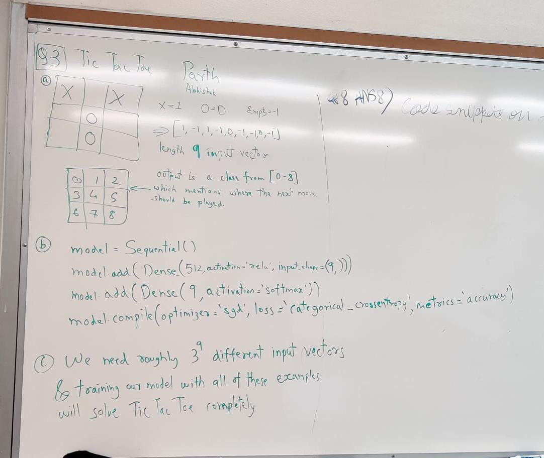
'''Q3) Answer 3)'''
((resource:WhatsApp Image 2021-12-06 at 8.59.07 PM.jpeg|Resource Description for WhatsApp Image 2021-12-06 at 8.59.07 PM.jpeg))
Manasa Mananjaya, Prajna Puranik
7. Give one adaptive learning rate algorithm for neural nets that we considered in class and motivate how it works.
Solution:
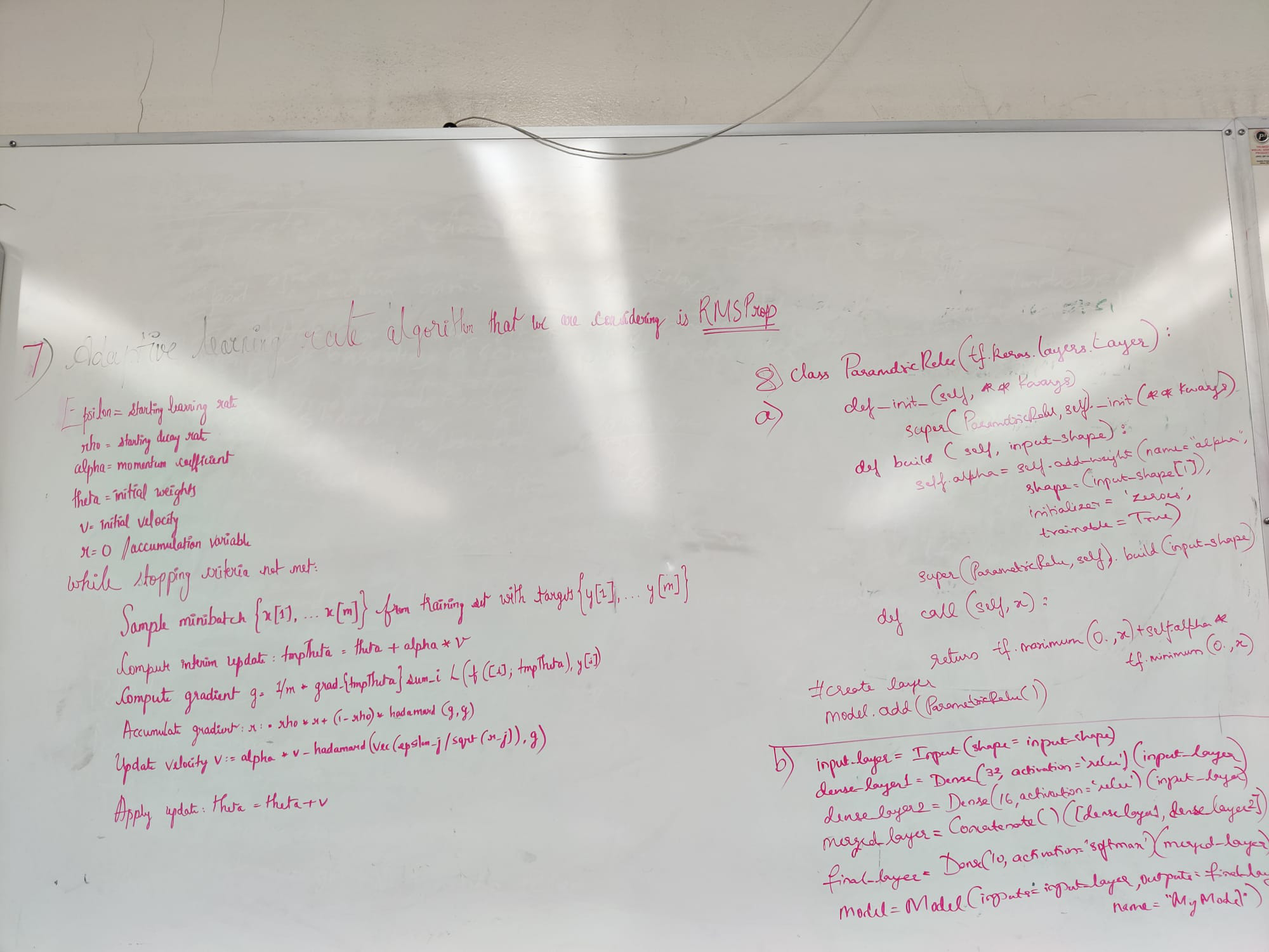
RMSProp modifies AdaGrad to use an exponentially decaying average of the gradient histories. It can be adapted to work with momentum and has been shown to work better with deep neural nets. Here is what the algorithm with Nestorov Momentum looks like:
RMSProp modifies AdaGrad to use an exponentially decaying average of the gradient histories. It can be adapted to work with momentum and has been shown to work better with deep neural nets. Here is what the algorithm with Nestorov Momentum looks like:
epsilon := starting learning rate
rho := starting decay rate
alpha := momentum coefficient
theta := initial weights
v := initial velocity
r := 0 // accumulation variable
while stopping criteria not met:
    Sample minibatch {x[1], ..., x[m]}
        from training set with targets {y[1], ..., y[m]}.
    Compute interim update: tmpTheta := theta + alpha*v
    Compute gradient g := 1/m * grad_{tmpTheta} sum_i L(f([i]; tmpTheta), y[i])
    Accumulate gradient: r := rho * r + (1 - rho)* hadamard (g, g)
        // pointwise product
    Update velocity: v := alpha * v - hadamard (vec (epsilon_j /sqrt(r_j)),  g)
        //make vector of epsilons then hadamard
    Apply update: theta := theta + v
8. Give a code example with explanation of how to create a custom layer in Keras. Give a code example of how to create a custom network topology using Keras' functinal API.
Solution:
Creating a Parametric ReLU layer as a custom layer using Keras:
Solution:
Creating a Parametric ReLU layer as a custom layer using Keras:
import tensorflow as tf
class ParametricRelu(tf.keras.layers.Layer):
Given a Sequential model, we could then add this layer using:
model.add(ParametricRelu());
    def __init__(self, **kwargs):
        # constructor here is calling the parent
        super(ParametricRelu, self).__init__(**kwargs)
    # in build below we specify one new weight to train with initial value 0
    # we also say this layer's units only take 1 input
    def build(self, input_shape):
        self.alpha = self.add_weight(
            name = 'alpha', shape=(input_shape[1]),
            initializer = 'zeros',
            trainable = True
        )
        super(ParametricRelu, self).build(input_shape)
    # for the inputs to a unit (in this case just 1), how we compute the output of that unit
    def call(self, x):
        return tf.maximum(0.,x)+ self.alpha * tf.minimum(0.,x)
Given a Sequential model, we could then add this layer using:
model.add(ParametricRelu());
Example of how to create a custom network topology using Keras' functinal API.
input_layer = Input(shape=input_shape)
take all inputs and feeds to 32 neurons
dense_layer_1 = Dense(32, activation='relu')(input_layer)
take all inputs and feeds to 16 neurons
dense_layer_2 = Dense(16, activation='relu')(input_layer)
makes a single layer with above two layers happening in parallel
merged_layer = Concatenate()([dense_layer_1, dense_layer_2])
feeds results of layer into a final layer
final_layer = Dense(10, activation='softmax')(merged_layer)
create model specifying input and output layers.
model = Model(inputs=input_layer, outputs=final_layer, name="My Model")
9. Give the back-propagation through time algorithm. Explain the teaching-forcing algorithm. Explain the long term dependency problem and why LSTMs might help to solve this problem.
solution:
a. To compute the gradient of the just presented network involves performing a forward pass moving left to right through the unrolled computation graph. This is then followed by a backward propagation pass moving right to left through the graph. Together this gives a runtime of O(τ) and a memory cost of O(τ). This process is called back-propagation through time (BPTT) and can be very expensive because it can't be easily parallelized as the forward graph is sequential in nature and we need to remember each value for the backward pass.
c.Long term dependencies can cause problems while training with RNN, which is that unfolding them multiple steps can have the effect of matrix powering. To avoid long term dependencies, LSTMs make use of a memory cell which can remember the previous state. Unlike normal RNNs, this cell's value is also controlled by forget lines that can roughly reset the memory of the previous state to 0, thus, preventing the powering issue.
(Edited: 2021-12-06) solution:
a. To compute the gradient of the just presented network involves performing a forward pass moving left to right through the unrolled computation graph. This is then followed by a backward propagation pass moving right to left through the graph. Together this gives a runtime of O(τ) and a memory cost of O(τ). This process is called back-propagation through time (BPTT) and can be very expensive because it can't be easily parallelized as the forward graph is sequential in nature and we need to remember each value for the backward pass.
b. Teacher forcing algorithm implements an RNN that produces an output at each time step and has recurrent connections only from the outputs at one step to the hidden units at the next. Rather than feeding the model's own output back into itself during training, it uses the sequence x⃗ (1),...,x⃗ (t) so far, y⃗ (t) and y⃗ (t−1), where y⃗ (t−1 )acts as a teacher forcing what the previous answer should be.
c.Long term dependencies can cause problems while training with RNN, which is that unfolding them multiple steps can have the effect of matrix powering. To avoid long term dependencies, LSTMs make use of a memory cell which can remember the previous state. Unlike normal RNNs, this cell's value is also controlled by forget lines that can roughly reset the memory of the previous state to 0, thus, preventing the powering issue.
Manasa Mananjaya, Prajna Puranik<br><br>
'''7. Give one adaptive learning rate algorithm for neural nets that we considered in class and motivate how it works.'''
<u>Solution:</u>
<br>
RMSProp modifies AdaGrad to use an exponentially decaying average of the gradient histories. It can be adapted to work with momentum and has been shown to work better with deep neural nets. Here is what the algorithm with Nestorov Momentum looks like:
<br>
''epsilon := starting learning rate<br>
rho := starting decay rate<br>
alpha := momentum coefficient<br>
theta := initial weights<br>
v := initial velocity<br>
r := 0 // accumulation variable <br>
while stopping criteria not met:<br>
Sample minibatch {x[1], ..., x[m]}
from training set with targets {y[1], ..., y[m]}.
Compute interim update: tmpTheta := theta + alpha*v
Compute gradient g := 1/m * grad_{tmpTheta} sum_i L(f([i]; tmpTheta), y[i])
Accumulate gradient: r := rho * r + (1 - rho)* hadamard (g, g)
// pointwise product
Update velocity: v := alpha * v - hadamard (vec (epsilon_j /sqrt(r_j)), g)
//make vector of epsilons then hadamard
Apply update: theta := theta + v
''
'''8.''' '''Give a code example with explanation of how to create a custom layer in Keras. Give a code example of how to create a custom network topology using Keras' functinal API.'''<br>
<u>Solution:</u> <br>Creating a Parametric ReLU layer as a custom layer using Keras:<br>
import tensorflow as tf
class ParametricRelu(tf.keras.layers.Layer):
def __init__(self, **kwargs):
# constructor here is calling the parent
super(ParametricRelu, self).__init__(**kwargs)
# in build below we specify one new weight to train with initial value 0
# we also say this layer's units only take 1 input
def build(self, input_shape):
self.alpha = self.add_weight(
name = 'alpha', shape=(input_shape[1]),
initializer = 'zeros',
trainable = True
)
super(ParametricRelu, self).build(input_shape)
# for the inputs to a unit (in this case just 1), how we compute the output of that unit
def call(self, x):
return tf.maximum(0.,x)+ self.alpha * tf.minimum(0.,x)
<br>
Given a Sequential model, we could then add this layer using:<br>
model.add(ParametricRelu());<br><br>
Example of how to create a custom network topology using Keras' functinal API.
<br>
#input_layer = Input(shape=input_shape)
#take all inputs and feeds to 32 neurons
dense_layer_1 = Dense(32, activation='relu')(input_layer)
#take all inputs and feeds to 16 neurons
dense_layer_2 = Dense(16, activation='relu')(input_layer)
#makes a single layer with above two layers happening in parallel
merged_layer = Concatenate()([dense_layer_1, dense_layer_2])
#feeds results of layer into a final layer
final_layer = Dense(10, activation='softmax')(merged_layer)
#create model specifying input and output layers.
model = Model(inputs=input_layer, outputs=final_layer, name="My Model")
<br><br>
9. '''Give the back-propagation through time algorithm. Explain the teaching-forcing algorithm. Explain the long term dependency problem and why LSTMs might help to solve this problem.'''<br>
<br><u>solution:</u><br>
<br>
a. To compute the gradient of the just presented network involves performing a forward pass moving left to right through the unrolled computation graph. This is then followed by a backward propagation pass moving right to left through the graph. Together this gives a runtime of O(τ) and a memory cost of O(τ). This process is called back-propagation through time (BPTT) and can be very expensive because it can't be easily parallelized as the forward graph is sequential in nature and we need to remember each value for the backward pass.
<br>
b. Teacher forcing algorithm implements an RNN that produces an output at each time step and has recurrent connections only from the outputs at one step to the hidden units at the next. Rather than feeding the model's own output back into itself during training, it uses the sequence x⃗ (1),...,x⃗ (t) so far, y⃗ (t) and y⃗ (t−1), where y⃗ (t−1 )acts as a teacher forcing what the previous answer should be.<br><br>
c.Long term dependencies can cause problems while training with RNN, which is that unfolding them multiple steps can have the effect of matrix powering. To avoid long term dependencies, LSTMs make use of a memory cell which can remember the previous state. Unlike normal RNNs, this cell's value is also controlled by forget lines that can roughly reset the memory of the previous state to 0, thus, preventing the powering issue.
<br><br>
((resource:WhatsApp Image 2021-12-06 at 5.29.31 PM.jpeg|Resource Description for WhatsApp Image 2021-12-06 at 5.29.31 PM.jpeg))
Divyaraj & Shashwat
Question-2:
Gradient descent is an iterative algorithm, that starts from a random point on a function and travels down its slope in steps until it reaches the lowest point of that function.
Gradient Descent Algorithm:
- Step 1: We calculate the slope of the loss function with respect to each feature.
- Step 2: Pick random parameters initially
- Step 3: Update the gradient function with parameters
- Step 4: Calculate the step size = learning rate * gradient
- Step 5: Calculate new parameters as new params = old params - step size
- Step 6: Repeat steps till gradient reaches zero or reaches the iteration limit
In Batch Gradient Descent , at each step of the gradient descent we use the whole data to compute the loss. The overall complexity to calculate the loss is O(m) where m is the number of instances in the dataset. This is a poor model because the dataset may contain thousands of training examples. So the training will be very slow.
In Stochastic Gradient Descent , at each step of the gradient descent rather than compute the complete sum, we can sample a minibatch, 𝔹={x(1),...,x(m′)} drawn uniformly from the training set. This overall reduces the number of instances to calculate the loss. Because the batches are drawn at random, the loss calculated over the mini batch will be representative to the whole dataset.
In Online Gradient Descent , at each step of the gradient descent we take a mini batch of size 1.
(Edited: 2021-12-06) Divyaraj & Shashwat
Question-2:
Gradient descent is an iterative algorithm, that starts from a random point on a function and travels down its slope in steps until it reaches the lowest point of that function.
'''Gradient Descent Algorithm:
'''
* Step 1: We calculate the slope of the loss function with respect to each feature.
* Step 2: Pick random parameters initially
* Step 3: Update the gradient function with parameters
* Step 4: Calculate the step size = learning rate * gradient
* Step 5: Calculate new parameters as new params = old params - step size
* Step 6: Repeat steps till gradient reaches zero or reaches the iteration limit
In '''Batch Gradient Descent''', at each step of the gradient descent we use the whole data to compute the loss. The overall complexity to calculate the loss is O(m) where m is the number of instances in the dataset. This is a poor model because the dataset may contain thousands of training examples. So the training will be very slow.
In '''Stochastic Gradient Descent''', at each step of the gradient descent rather than compute the complete sum, we can sample a minibatch, 𝔹={x(1),...,x(m′)} drawn uniformly from the training set. This overall reduces the number of instances to calculate the loss. Because the batches are drawn at random, the loss calculated over the mini batch will be representative to the whole dataset.
In '''Online Gradient Descent''', at each step of the gradient descent we take a mini batch of size 1.
Tarun Mourya Satveli
Venkata Sai Sathwik Nadella
Question 1.
Question 9. a) A forward pass through the unrolled computation graph from left to right is required to calculate the gradient of the network. This is then followed by a backward propagation pass Overall, this gives a runtime of O(τ) and a memory cost of O(τ) which is called back-propagation through time (BPTT)
b) The Teacher Forcing algorithm trains recurrent networks by supplying observed sequence values as inputs during training and using the network's own one-step-ahead predictions to do multi-step sampling. We introduce the Professor Forcing algorithm, which uses adversarial domain adaptation to encourage the dynamics of the recurrent network to be the same when training the network and when sampling from the network over multiple time steps.
c) One issue with RNN training is that unfolding them in several steps can result in matrix powering. If we suppose that our activation function is the same as our activation function, then computing an RNN layer yields a recurrence like:
If W has an eigenvalue decomposition, then W=QΛQ−1, where Λ is a diagonal matrix, so the above becomes:
h⃗ (t)=(Q−1ΛtQ)h⃗ (0)
and we see if the largest magnitude of W's eigenvalues is greater than 1, the value of h will tend to explode, and if it's less than 1 the values will tend to go 0 rapidly.
It can be hard to train RNNs if τ is large
To avoid long term dependencies, LSTMs make use of a memory cell which can remember the previous state.
Unlike normal RNNs, this cell's value is also controlled by forget lines that can roughly reset the memory of the previous state to 0, thus, preventing the powering issue
(Edited: 2021-12-06) Tarun Mourya Satveli
Venkata Sai Sathwik Nadella
Question 1.
((resource:image (1).png|Resource Description for image (1).png))
Question 9. a) A forward pass through the unrolled computation graph from left to right is required to calculate the gradient of the network. This is then followed by a backward propagation pass Overall, this gives a runtime of O(τ) and a memory cost of O(τ) which is called back-propagation through time (BPTT)
b) The Teacher Forcing algorithm trains recurrent networks by supplying observed sequence values as inputs during training and using the network's own one-step-ahead predictions to do multi-step sampling. We introduce the Professor Forcing algorithm, which uses adversarial domain adaptation to encourage the dynamics of the recurrent network to be the same when training the network and when sampling from the network over multiple time steps.
c) One issue with RNN training is that unfolding them in several steps can result in matrix powering. If we suppose that our activation function is the same as our activation function, then computing an RNN layer yields a recurrence like:
((resource:Screen Shot 2021-12-06 at 4.39.03 PM.png|Resource Description for Screen Shot 2021-12-06 at 4.39.03 PM.png))
If W has an eigenvalue decomposition, then W=QΛQ−1, where Λ is a diagonal matrix, so the above becomes:
'''h⃗ (t)=(Q−1ΛtQ)h⃗ (0)'''
and we see if the largest magnitude of W's eigenvalues is greater than 1, the value of h will tend to explode, and if it's less than 1 the values will tend to go 0 rapidly.
It can be hard to train RNNs if τ is large
To avoid long term dependencies, LSTMs make use of a memory cell which can remember the previous state.
Unlike normal RNNs, this cell's value is also controlled by forget lines that can roughly reset the memory of the previous state to 0, thus, preventing the powering issue
Q 10:
Shashwat Kadam.
Divyaraj Chauhan
Ng's Neural net design methodology:
- Determine the problem to solve and metrics by which to measure success.
- Develop an architecture including training algorithms.
- Instrument the system to determine bottleneck/performance issues and their causes
- Incrementally make changes to the modes, collect new data, adjust hyperparameters.
Step 1: Determining the problem to solve and choosing the metrics to evaluate it.
The first step to solving the problem is to understand all the fine details of it and figure out the way to tackle it. For example, if we have to recognize a handwritten number from an MNIST dataset, we have to first figure out all the details of the dataset. The dataset contains 60000 images each of size 28 X 28. As the images are fairly small for computation, we can then decide whether to choose a fully connected neural network with two or three layers. But using convolutional neural networks can help learn the features like 'loops' and 'edges' in the images and also reduce the complexity of the network.
Another task is to choose how many layers will the network have and how many neurons (kernels) each layer will have. Once we figure this out and train our model, we must find a way to evaluate the model. One way to do it is by a confusion matrix where we know the Rate of false positives and correct predictions.
Q 10:
Shashwat Kadam.
Divyaraj Chauhan
Ng's Neural net design methodology:
# '''Determine the problem to solve and metrics by which to measure success.'''
# '''Develop an architecture including training algorithms.'''
# '''Instrument the system to determine bottleneck/performance issues and their causes'''
# '''Incrementally make changes to the modes, collect new data, adjust hyperparameters.'''
Step 1: Determining the problem to solve and choosing the metrics to evaluate it.
The first step to solving the problem is to understand all the fine details of it and figure out the way to tackle it. For example, if we have to recognize a handwritten number from an MNIST dataset, we have to first figure out all the details of the dataset. The dataset contains 60000 images each of size 28 X 28. As the images are fairly small for computation, we can then decide whether to choose a fully connected neural network with two or three layers. But using convolutional neural networks can help learn the features like 'loops' and 'edges' in the images and also reduce the complexity of the network.
Another task is to choose how many layers will the network have and how many neurons (kernels) each layer will have. Once we figure this out and train our model, we must find a way to evaluate the model. One way to do it is by a confusion matrix where we know the Rate of false positives and correct predictions.
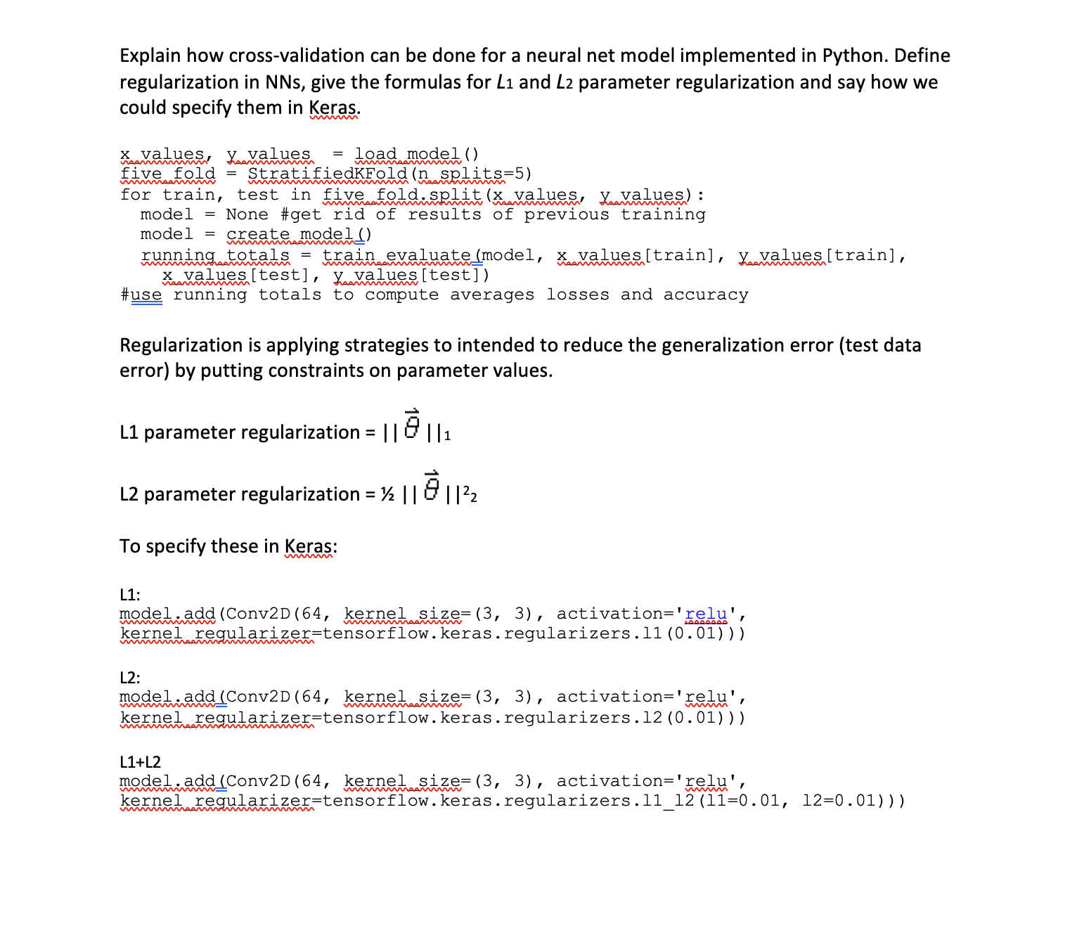
Rishabh Pandey, Madhujita Ambaskar
(Edited: 2021-12-06) ((resource:cross.png|Resource Description for cross.png))
Rishabh Pandey, Madhujita Ambaskar
Rishabh Pandey, Madhujita Ambaskar
Problem 9:
Backpropagation through time (BPTT) is a gradient-based technique for training certain types of recurrent neural networks.
To compute the gradient of the network we perform a forward pass moving left to right through the unrolled computation graph and then perform a backward propagation pass moving right to left through the graph. The whole process is called Back Propagation through Time algorithm.
Teacher Forcing Training:
In the second RNN design pattern which produces an output at each time step and has recurrent connections only from the outputs at one step to the hidden units at the next. Teacher forcing is a method for quickly and efficiently training recurrent neural network models that use the ground truth from a prior time step as input.
long Term Dependency Problem: RNN can effect of matrix powering. A RNN can connect previous information to the present task.
Sometimes, we only need to look at recent information to perform the present task. For example, consider a language model trying to predict the next word based on the previous ones. If we are trying to predict the last word in “the clouds are in the sky,” we don’t need any further context – it’s pretty obvious the next word is going to be sky.
LSTM are a special kind of RNN, capable of solving learning long-term dependencies problem. LSTMs make use of a memory cell which can remember the previous state.
A diagram for LSTM is shown below:
(Edited: 2021-12-06) Rishabh Pandey, Madhujita Ambaskar
Problem 9:
Backpropagation through time (BPTT) is a gradient-based technique for training certain types of recurrent neural networks.
To compute the gradient of the network we perform a forward pass moving left to right through the unrolled computation graph and then perform a backward propagation pass moving right to left through the graph. The whole process is called Back Propagation through Time algorithm.
Teacher Forcing Training:
In the second RNN design pattern which produces an output at each time step and has recurrent connections only from the outputs at one step to the hidden units at the next. Teacher forcing is a method for quickly and efficiently training recurrent neural network models that use the ground truth from a prior time step as input.
long Term Dependency Problem: RNN can effect of matrix powering. A RNN can connect previous information to the present task.
Sometimes, we only need to look at recent information to perform the present task. For example, consider a language model trying to predict the next word based on the previous ones. If we are trying to predict the last word in “the clouds are in the sky,” we don’t need any further context – it’s pretty obvious the next word is going to be sky.
LSTM are a special kind of RNN, capable of solving learning long-term dependencies problem. LSTMs make use of a memory cell which can remember the previous state.
A diagram for LSTM is shown below:
((resource:WhatsApp Image 2021-12-06 at 5.26.44 PM.jpeg|Resource Description for WhatsApp Image 2021-12-06 at 5.26.44 PM.jpeg))
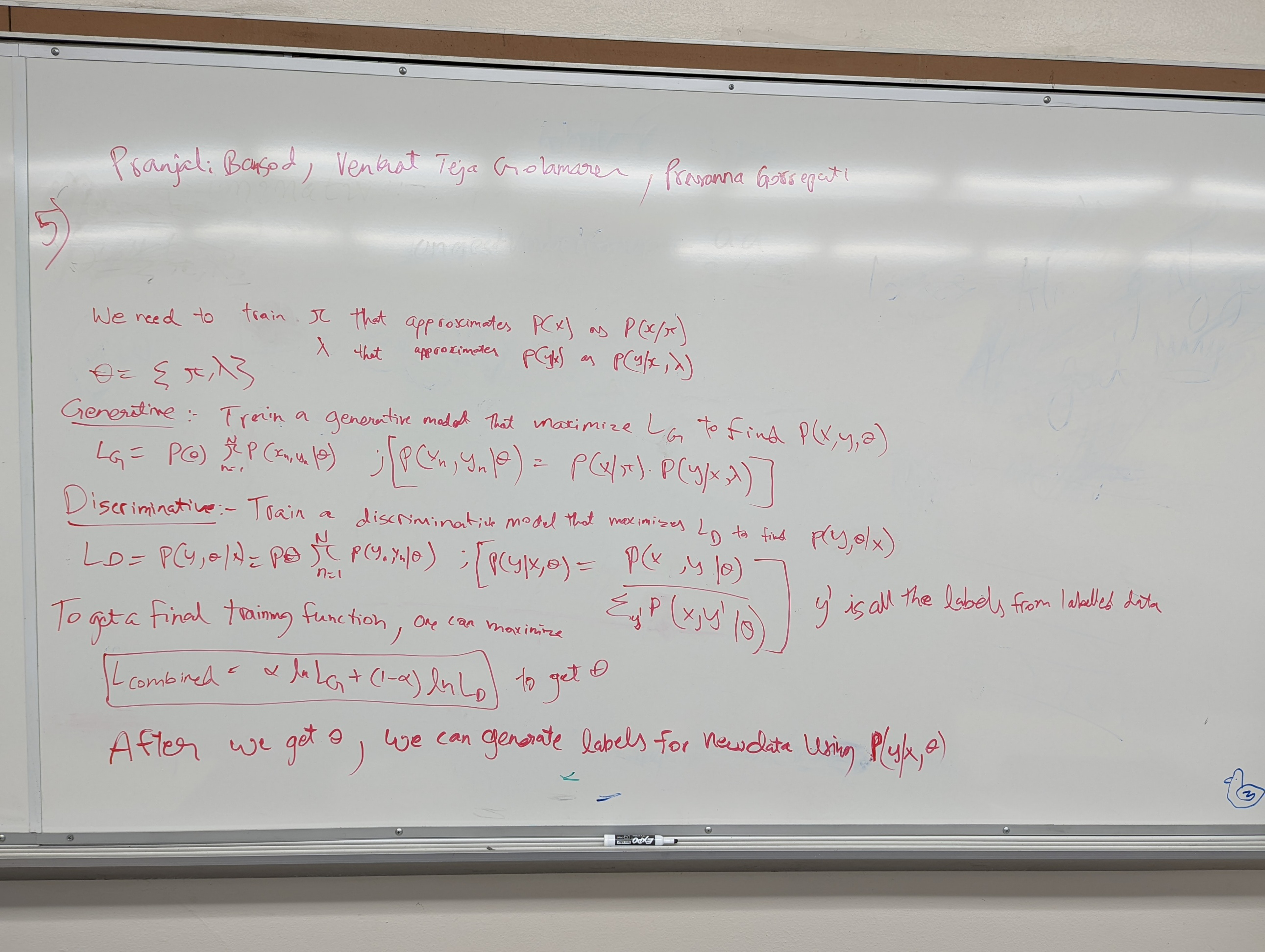
Venkat Teja Golamaru, Pranjali Bansod, Prasanna Gorrepati
Question 5
Question 8
This was the custom layer code used in HW4 using Keras.
class customConv2d(tflayers.Layer):
    def __init__(self, filters = None, filter_size = 5, kernel_type = '5square', model_regularizer = None,  **kwargs):
        self.filters = filters
        self.kernel_type = kernel_type
        self.kernel_size = [filter_size,filter_size]
        self.model_regularizer = model_regularizer
        super(customConv2d, self).__init__(**kwargs)

    def build(self, input_shape):
        shape = list(self.kernel_size) + [input_shape[-1], self.filters]
        self.kernel = self.add_weight(
            name = "kernel",
            shape=shape,
            initializer = 'glorot_uniform' if self.kernel_type == '5square' else diamond_kernel,
            regularizer = self.model_regularizer,
            trainable = True
        )

        weights = self.kernel.numpy()
        super(customConv2d, self).build(input_shape)
        return self.kernel
    def call(self, inputs):
        return K.conv2d(inputs, self.kernel)

    def get_config(self):
        config = super().get_config().copy()
        config.update({
            'filters': self.filters})
        return config
This is how we used that custom layer to build a LeNet model in Keras.
def LeNET():
(Edited: 2021-12-08)
    ip = tflayers.Input(shape=(32, 32, 3))
    c1 = customConv2d(6, 5, kernel_type, model_regularizer)(ip)
    c1 = tflayers.Activation('relu')(c1)
    cm1 = tflayers.MaxPooling2D((2, 2))(c1)
    c2 = customConv2d(16, 5, kernel_type, model_regularizer)(cm1)
    c2 = tflayers.Activation('relu')(c2)
    cm2 = tflayers.MaxPooling2D((2, 2))(c2)
    c3 = customConv2d(120, 5, kernel_type, model_regularizer)(cm2)
    c3 = tflayers.Activation('relu')(c3)
    if topology=='2':
        cm2_2 = tflayers.MaxPooling2D((6, 6))(c2)
        c3 = tflayers.Concatenate()([c3, cm2_2])

    flatten = tflayers.Flatten()(c3)
    dense = tflayers.Dense(84, activation='relu')(flatten)
    op = tflayers.Dense(4, activation='softmax')(dense)
    model = tf.keras.Model(ip, op, name = 'LeNet5_'+topology)
    model.compile(optimizer=model_optimizer, loss=tf.keras.losses.SparseCategoricalCrossentropy(), metrics=['acc'])
    print("Finished creating model", 'LeNet5_'+topology)
    return model
Venkat Teja Golamaru, Pranjali Bansod, Prasanna Gorrepati
Question 5
((resource:messages_0.jpeg|Resource Description for messages_0.jpeg))
Question 8
This was the custom layer code used in HW4 using Keras.
class customConv2d(tflayers.Layer):
def __init__(self, filters = None, filter_size = 5, kernel_type = '5square', model_regularizer = None, **kwargs):
self.filters = filters
self.kernel_type = kernel_type
self.kernel_size = [filter_size,filter_size]
self.model_regularizer = model_regularizer
super(customConv2d, self).__init__(**kwargs)
def build(self, input_shape):
shape = list(self.kernel_size) + [input_shape[-1], self.filters]
self.kernel = self.add_weight(
name = "kernel",
shape=shape,
initializer = 'glorot_uniform' if self.kernel_type == '5square' else diamond_kernel,
regularizer = self.model_regularizer,
trainable = True
)
weights = self.kernel.numpy()
super(customConv2d, self).build(input_shape)
return self.kernel
def call(self, inputs):
return K.conv2d(inputs, self.kernel)
def get_config(self):
config = super().get_config().copy()
config.update({
'filters': self.filters})
return config
This is how we used that custom layer to build a LeNet model in Keras.
def LeNET():
ip = tflayers.Input(shape=(32, 32, 3))
c1 = customConv2d(6, 5, kernel_type, model_regularizer)(ip)
c1 = tflayers.Activation('relu')(c1)
cm1 = tflayers.MaxPooling2D((2, 2))(c1)
c2 = customConv2d(16, 5, kernel_type, model_regularizer)(cm1)
c2 = tflayers.Activation('relu')(c2)
cm2 = tflayers.MaxPooling2D((2, 2))(c2)
c3 = customConv2d(120, 5, kernel_type, model_regularizer)(cm2)
c3 = tflayers.Activation('relu')(c3)
if topology=='2':
cm2_2 = tflayers.MaxPooling2D((6, 6))(c2)
c3 = tflayers.Concatenate()([c3, cm2_2])
flatten = tflayers.Flatten()(c3)
dense = tflayers.Dense(84, activation='relu')(flatten)
op = tflayers.Dense(4, activation='softmax')(dense)
model = tf.keras.Model(ip, op, name = 'LeNet5_'+topology)
model.compile(optimizer=model_optimizer, loss=tf.keras.losses.SparseCategoricalCrossentropy(), metrics=['acc'])
print("Finished creating model", 'LeNet5_'+topology)
return model
(c) 2026 Yioop - PHP Search Engine