
2020-04-28
Apr 29 In-Class Exercise Thread .
Please post your solutions to the Apr 29 In-Class Exercise to this thread.
Best,
Chris
Please post your solutions to the Apr 29 In-Class Exercise to this thread.
Best,
Chris
2020-04-29

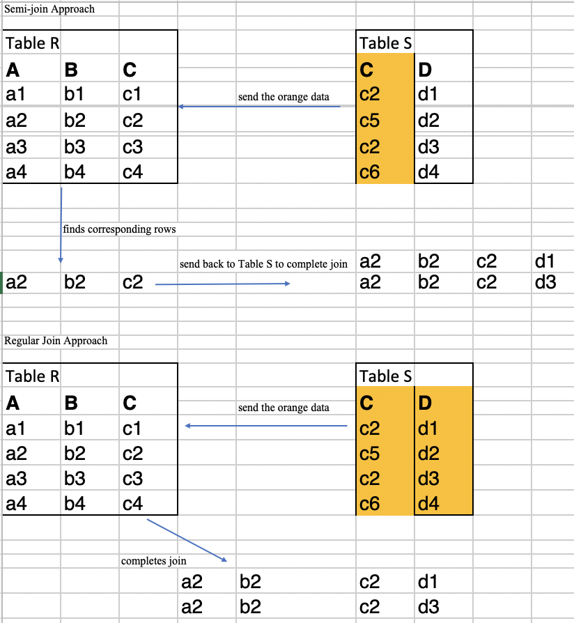
 Semi-join approach:
 - step 1: Table R's machine sends ("C" values: c1, c2, c3, c4) to table S
 - step 2: Table S's machine receives this information and sends corresponding rows( {c2, d1}, {c2, d3} )
 - step 3: Table R's machine receives this information and completes the join resulting in ( {a2, b2, c2, d1}, {a2, b2, c2, d3} )

 Send all S approach:
 - step 1: Table S's machine sends entire table ( {c2, d1}, {c5, d2}, {c2, d3}, {c6, d4} )
 - step 2: Table R's machine receives this information and does the join which results in ( {a2, b2, c2, d1}, {a2, b2, c2, d3} )

 In the first approach, we send 8 data items, but we must communicate twice between machines, while in the second approach we also send 8 data items, but there is only one communication between machines.
(Edited: 2020-04-29) Semi-join approach:
- step 1: Table R's machine sends ("C" values: c1, c2, c3, c4) to table S
- step 2: Table S's machine receives this information and sends corresponding rows( {c2, d1}, {c2, d3} )
- step 3: Table R's machine receives this information and completes the join resulting in ( {a2, b2, c2, d1}, {a2, b2, c2, d3} )
Send all S approach:
- step 1: Table S's machine sends entire table ( {c2, d1}, {c5, d2}, {c2, d3}, {c6, d4} )
- step 2: Table R's machine receives this information and does the join which results in ( {a2, b2, c2, d1}, {a2, b2, c2, d3} )
In the first approach, we send 8 data items, but we must communicate twice between machines, while in the second approach we also send 8 data items, but there is only one communication between machines.
TABLE R
A	B	C
a1	b1	c1
a2	b2	c2
a3	b3	c3
a4	b4	c4

TABLE S
C	D
c2	d1
c5	d2
c2	d3
c6	d4

First, we compute semi-join:
(S is on the left side because it's smaller.)
	S (SEMI-JOIN) R
Which evaluates to:
	S (NATURAL-JOIN) (PROJECT(R, C))
First, we perfrom (PROJECT(R, C)), which is: (The machine with R computes this) </pre>
(PROJECT(R, C))
C
c2
c5
c2
c6
Next, we join:
Bag join is assumed.
(The machine with S computes this)
Which evaluates to:
A   B   C
a2  b2  c2
a2  b2  c2
Next, we send this table to the machine with the table R, and we compute the final join. A B C D a2 b2 c2 d1 a2 b2 c2 d3(Edited: 2020-04-29)
<pre>
TABLE R
A B C
a1 b1 c1
a2 b2 c2
a3 b3 c3
a4 b4 c4
TABLE S
C D
c2 d1
c5 d2
c2 d3
c6 d4
First, we compute semi-join:
(S is on the left side because it's smaller.)
S (SEMI-JOIN) R
</pre><pre>
Which evaluates to:
S (NATURAL-JOIN) (PROJECT(R, C))
</pre>
First, we perfrom (PROJECT(R, C)), which is:
(The machine with R computes this)
</pre><pre>
(PROJECT(R, C))
C
c2
c5
c2
c6
</pre><pre>
Next, we join:
Bag join is assumed.
(The machine with S computes this)
Which evaluates to:
A B C
a2 b2 c2
a2 b2 c2
</pre><pre>
Next, we send this table to the machine with
the table R, and we compute the final join.
A B C D
a2 b2 c2 d1
a2 b2 c2 d3
</pre>
 Step 1: S sends over column C (4 entries)
 Step 2: R computes R semi-join S {[a2, b2, c2]} and sends that to S
 Step 3: S uses the result to compute the natural join {[a2, b2, c2, d1], [a2, b2, c2, d3]}
This method sends 4 entries over and then 3 entries back over (2 communications, 7 entries sent total) A traditional method would have S send over its entire table to R (1 communication, 8 entries sent total)(Edited: 2020-04-29)
Step 1: S sends over column C (4 entries)
Step 2: R computes R semi-join S {[a2, b2, c2]} and sends that to S
Step 3: S uses the result to compute the natural join {[a2, b2, c2, d1], [a2, b2, c2, d3]}
This method sends 4 entries over and then 3 entries back over (2 communications, 7 entries sent total)
A traditional method would have S send over its entire table to R (1 communication, 8 entries sent total)
Semi join:
R sends its C columns to S -> c1, c2, c3, c4
Do the join on S
Return rows: (c2, d1), (c2, d3)
R finishes with result:
(a2, b2, c2, d1), (a2, b2, c2, d3)
Total row entries moved: 8 (where ‘c1’ is a row entry and (c2, d1) are two row entries)
Naive approach:
Send all of table S to R: (c2,d1), (c5, d2), (c2, d3), (c6, d4)
R computes the join and finishes with result:
(a2, b2, c2, d1), (a2, b2, c2, d3)
Total row entries moved: 8
The total amount of data moved is the same, if the size of each entry is the same (say an integer). This is likely not to be the case in more real-world examples.
(Edited: 2020-04-29) Semi join:
R sends its C columns to S -> c1, c2, c3, c4
Do the join on S
Return rows: (c2, d1), (c2, d3)
R finishes with result:
(a2, b2, c2, d1), (a2, b2, c2, d3)
Total row entries moved: 8 (where ‘c1’ is a row entry and (c2, d1) are two row entries)
<br />
<br />
Naive approach:
Send all of table S to R: (c2,d1), (c5, d2), (c2, d3), (c6, d4)
R computes the join and finishes with result:
(a2, b2, c2, d1), (a2, b2, c2, d3)
Total row entries moved: 8
The total amount of data moved is the same, if the size of each entry is the same (say an integer). This is likely not to be the case in more real-world examples.
 Semi-join:
 S has the smaller table.
 1. Machine with R computes π_{C}(R) and sends it to S.
 π_{C}(R)= {c1, c2, c3, c4}
 2. Machine with S computes S⋉R sends it to the machine with R.
 S⋉R = {(c2, d1), (c2,d3)}
 3. Machine with R uses S⋉R to compute S(C,D)⋈R(A,B,C).
 S(C,D)⋈R(A,B,C) = {(a2,b2,c2,d1), (a2,b2,c2,d3)}

 Naive
 1. S has a smaller table.
 2. A copy of S is sent to R and the join is computed there.
 {(c2,d1), (c5, d2), (c2, d3), (c6, d4)} sent to R.
 R computes the join: R⋈S = {(a2, b2, c2, d1), (a2, b2, c2, d3)}

 The semi-join approach costs seven entries and two times of communication. The naive way costs 8 entries and one
 time of communication.
Semi-join:
S has the smaller table.
1. Machine with R computes π_{C}(R) and sends it to S.
π_{C}(R)= {c1, c2, c3, c4}
2. Machine with S computes S⋉R sends it to the machine with R.
S⋉R = {(c2, d1), (c2,d3)}
3. Machine with R uses S⋉R to compute S(C,D)⋈R(A,B,C).
S(C,D)⋈R(A,B,C) = {(a2,b2,c2,d1), (a2,b2,c2,d3)}
Naive
1. S has a smaller table.
2. A copy of S is sent to R and the join is computed there.
{(c2,d1), (c5, d2), (c2, d3), (c6, d4)} sent to R.
R computes the join: R⋈S = {(a2, b2, c2, d1), (a2, b2, c2, d3)}
The semi-join approach costs seven entries and two times of communication. The naive way costs 8 entries and one
time of communication.
Send all:
- step 1: The machine of table S sends to the machine of table R the whole table S( {c2, d1}, {c5, d2}, {c2, d3}, {c6, d4} )
- step 2: The machine of table R receives the information from table S and does the join with table S and results in ( {a2, b2, c2, d1}, {a2, b2, c2, d3} )
Semi-join:
- step 1: The machine of table R sends to the machine of table S only column C values ( c1, c2, c3, c4 )
- step 2: The machine of table S receives this information and does the semi-join on the column C, then it sends to the machine of table R the corresponding rows ( {c2, d1}, {c2, d3} )
- step 3: The machine of table R receives the information from the machine of table S and completes the join which results in ( {a2, b2, c2, d1}, {a2, b2, c2, d3} )
Compare:
The semi-join approach requires more communication between two machines than send all approach. If we assume the communication cost between two machines is not expensive then the semi-join approach would be better in this situation.
(Edited: 2020-04-29) Send all:
- step 1: The machine of table S sends to the machine of table R the whole table S( {c2, d1}, {c5, d2}, {c2, d3}, {c6, d4} )
- step 2: The machine of table R receives the information from table S and does the join with table S and results in ( {a2, b2, c2, d1}, {a2, b2, c2, d3} )
Semi-join:
- step 1: The machine of table R sends to the machine of table S only column C values ( c1, c2, c3, c4 )
- step 2: The machine of table S receives this information and does the semi-join on the column C, then it sends to the machine of table R the corresponding rows ( {c2, d1}, {c2, d3} )
- step 3: The machine of table R receives the information from the machine of table S and completes the join which results in ( {a2, b2, c2, d1}, {a2, b2, c2, d3} )
Compare:
The semi-join approach requires more communication between two machines than send all approach. If we assume the communication cost between two machines is not expensive then the semi-join approach would be better in this situation.
 -Step 1: S sends over column C, about 4 columns
 -Step 2: Computes R semi-join S {[a2, b2, c2]} and sends that to S
 -Step 3: S received the result and compute natural join {[a2, b2, c2, d1], [a2, b2, c2, d3]}
 -To compare:
  With semi-join, 7 columns are sent total where as with traditional method 8 columns are needed.
-Step 1: S sends over column C, about 4 columns
-Step 2: Computes R semi-join S {[a2, b2, c2]} and sends that to S
-Step 3: S received the result and compute natural join {[a2, b2, c2, d1], [a2, b2, c2, d3]}
-To compare:
With semi-join, 7 columns are sent total where as with traditional method 8 columns are needed.
2020-05-01
First R would send to S its matching attribute column C with the values that might join with S: c1, c2, c3, c4. Then S computes the join and sends it to R: (c2, d1), (c2, d3). Then R uses that to compute the join: (a2, b2, c2, d1), (a2, b2, c2, d3).
A comparison of this method versus just simply sending over all of S is that we have more communication overhead because we need to send data two times(first the potential columns that may join, then the semi-join) instead of just once. For this current example, 3 columns are being sent for the semi-join method whereas just sending over S would have sent 2 columns.(Edited: 2020-05-01)
<pre> First R would send to S its matching attribute column C with the values that might join with S: c1, c2, c3, c4. Then S computes the join and sends it to R: (c2, d1), (c2, d3). Then R uses that to compute the join: (a2, b2, c2, d1), (a2, b2, c2, d3). </pre>
<pre> A comparison of this method versus just simply sending over all of S is that we have more communication overhead because we need to send data two times(first the potential columns that may join, then the semi-join) instead of just once. For this current example, 3 columns are being sent for the semi-join method whereas just sending over S would have sent 2 columns.</pre>
2020-05-02
The semi-join method sends 7 entries in total. The regular join method sends 8 entries in total. In this case, the semi-join is more efficient than the regular join.
((resource:Screen Shot 2020-05-02 at 6.31.46 PM.png|Resource Description for Screen Shot 2020-05-02 at 6.31.46 PM.png))
The semi-join method sends 7 entries in total. The regular join method sends 8 entries in total. In this case, the semi-join is more efficient than the regular join.
(c) 2026 Yioop - PHP Search Engine